
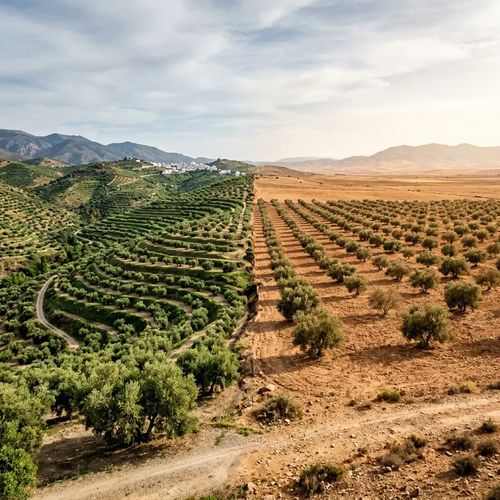
This spring the preliminary harvest estimates for 26/27 are pointing upwards. Generous October-April rainfall, reservoirs well recovered —Seville at 83 %, Huelva at 87 %—, spring NDVI at high levels. Estimate: a good harvest.
It is worth pausing before trusting that. In the spring of 2022 Andalusia’s NDVI was at the same level as any good year (0.406, the same as 2020, which gave 1,181 kt across the eight large olive-growing provinces). Then summer came, the thermometer shot up, and the harvest fell to 666 kt: 55 % less. And in 2024, with reservoirs at almost the same low level as in 2022 (39 % against 37 %), the harvest closed above 1,250 kt because the summer was mild.
When the first version of this analysis stayed at Andalusian provincial scale with five comparable seasons, one story came out: May-to-July heat was the strongest predictor. But when we widened the exercise to twenty-five years of data and nine olive-growing countries, that story becomes richer and, in some respects, different. There is no single model of the Mediterranean olive tree. What decides the harvest in Spain is not the same as in Italy, in Tunisia or in Morocco. That is what this article is about.
A note on method before we start. Annual national production comes from the International Olive Council (IOC), 2000-2024 series by country. Climate comes from daily data processed by Olearia Intelligence, aggregated to the year or to the relevant phenological window. Correlations are Pearson; R² values are simple and built incrementally to avoid attributing the same effect twice. When a variable becomes irrelevant after controlling for an earlier one, we say so.
What decides the harvest in Spain: January-to-April water
Let’s start at home. Spain produces 1.2 Mt a year on average, with brutal swings —from 618 kt in 2012/13 to 1,790 kt in 2018/19—, and twenty-five years of history to ask the data what explains those swings.
| Series | 2000 | 2001 | 2002 | 2003 | 2004 | 2005 | 2006 | 2007 | 2008 | 2009 | 2010 | 2011 | 2012 | 2013 | 2014 | 2015 | 2016 | 2017 | 2018 | 2019 | 2020 | 2021 | 2022 | 2023 | 2024 |
|---|---|---|---|---|---|---|---|---|---|---|---|---|---|---|---|---|---|---|---|---|---|---|---|---|---|
| Production (kt) | 974 | 1411 | 861 | 1412 | 990 | 827 | 1111 | 1236 | 1030 | 1402 | 1392 | 1615 | 618 | 1782 | 842 | 1403 | 1291 | 1262 | 1790 | 1125 | 1389 | 1492 | 666 | 855 | 1419 |
| Jan-Apr rainfall (mm × 5) | 645 | 1060 | 830 | 1155 | 1185 | 420 | 980 | 930 | 970 | 990 | 1870 | 1065 | 455 | 1585 | 1065 | 810 | 980 | 810 | 1830 | 650 | 1110 | 1085 | 1205 | 355 | 1540 |
You can see it at a glance. The catastrophic 2022 harvest (666 kt) coincides with one of the century’s worst January-to-Aprils for rain. The 1,790 kt record in 2018 coincides with a very generous hydrological winter. The correlation between January-April rainfall and national production is +0.64 over twenty-five years.
It is robust. It holds if we remove the two extremes (the 2018 record and the 2022 low): r=+0.64. It holds in 2000-2010 (r=+0.63), in 2011-2020 (r=+0.87) and in 2015-2024 (r=+0.62). It is not an artefact of a couple of odd years: it is a structural signal.
In more useful terms: winter rainfall explains 41 % of the year-to-year variance of the Spanish harvest. For a single variable with n=25 in a biological system as noisy as an olive grove, that is a great deal.
What about reservoirs? Much less than it seems
For years the sector has talked about Andalusia’s reservoirs as if they were the main gauge of the next harvest. Seville at 83 %, Huelva at 87 %, Jaén at 65 %. When the numbers go up, optimism; when they go down, alarm. But the data tell a different story.
We tested reservoir level —aggregate of five Andalusian olive-growing provinces, weekly data 2000-2024, hydrological year— as a predictor of the national harvest. The raw correlation is +0.34 to +0.36, weak but positive. If we build a linear model that first captures the effect of rainfall and then asks how much the reservoir adds, the reservoir contributes only 2 % additional explained variance. The reverse does happen: rainfall, after removing the reservoir, still contributes 31 %.
Why? Because rainfall and reservoirs, contrary to appearances, are not the same thing at national scale. Their correlation with each other is only +0.14: there are years of abundant rain with low reservoirs (drawn down by irrigation of earlier crops) and years of scarce rain with high reservoirs (left over from the previous winter). Rain-fed olive groves, which are the bulk of Spain’s olive groves, are not irrigated from reservoirs. They are watered by the rain that falls directly on the plot. Only intensive irrigated groves depend on reservoirs, and they are a minority of national volume.
The uncomfortable conclusion: reservoirs are a media indicator, not a statistical one. Visible, easy to photograph and easy to comment on in the press. But as a predictor of the national harvest, direct rainfall over the olive-growing provinces is four times more informative.
Heat does matter, but as an interaction
The first version of this analysis, done only at provincial scale with five seasons, said that May-to-July heat stress was the dominant predictor. With twenty-five national years that reading changes, but not in the simple way we expected.
The raw correlation between days of extreme heat in May-July and production is −0.19, weak but negative. That of the average maximum temperature is −0.31. Three indicators pointing the same way: when it is hotter, the harvest falls. So far, consistent with physiology.
The problem appears when we build an additive linear model —first rainfall, then heat on top as an independent term—. After rainfall, maximum temperature adds 0.2 % more. Vapour pressure deficit, 0.1 %. Almost zero. Read carelessly, that would suggest heat does not matter. And that would be a mistake.
What happens is that the effect of heat is not additive, it is multiplicative. It depends on how much water the tree had when the heat arrived. Look at this table, built by splitting the 25 years of data into hydrological and thermal regimes:
| Jan-Apr rainfall / June tmax | Cool summer | Mild summer | Hot summer |
|---|---|---|---|
| Dry year | 1,236 kt | 1,044 kt | 902 kt |
| Normal year | 1,162 kt | 1,335 kt | 1,351 kt |
| Wet year | 1,554 kt | — | 1,023 kt |
Average national harvest in kt by regime, terciles of January-April rainfall and of June tmax. Twenty-five years, Spain. Source: IOC and Olearia Intelligence.
Look at the “wet year” row. With a cool summer it gives 1,554 kt —the big records—. With a hot summer it falls to 1,023 kt —a mediocre harvest, despite plentiful rain—. The difference between raining well and harvesting well is made by the summer. Heat does kill harvests, but only when the tree had water available and burned through it. When there was no water to begin with, heat no longer matters because the harvest was lost anyway.
That is what an additive linear model does not capture. And it is what non-linear techniques —such as carefully controlled Gradient Boosting— can capture. When we train a model of that kind with three selected variables (January-April rainfall, June tmax, previous year’s harvest) and evaluate it with honest cross-validation, it reaches R²=0.61 — twice what linear regression on rainfall alone gives. The difference is exactly the interaction that the regime table shows.
There is a second factor that also contributes: year-to-year persistence. If last year’s harvest was bad, the next one tends to be worse too. The correlation of production with the previous year’s is −0.30 on its own, and rises to −0.40 after controlling for rainfall. It is not noise: it is a real, complementary signal.
An important caveat: this persistence effect is not alternate bearing in the strict sense. Alternate bearing is the biennial cycle of the individual tree; an olive tree that yields a lot one year depletes its reserves and yields little the next. That happens at plot scale. At country scale, with millions of trees out of phase with each other, individual alternate bearing cancels out in the aggregate. What we measure when we correlate national production with itself is year-to-year autocorrelation: climate shocks that last more than a year, tree damage that takes time to repair, multi-year cycles of the olive stock. It is real and predictive, but calling it alternate bearing would be technically imprecise.
Three families of olive tree in the Mediterranean
Repeating the exercise in each large Mediterranean country is where the really interesting part appears. Twenty-two years, same method, eight countries with complete data:
| Country | Winter rain (R²) | Persistence (R²) | May-Jul heat (R²) | Dominant predictor |
|---|---|---|---|---|
| Spain | 41 % | 9 % | 9 % | Water |
| Morocco | 41 % | 47 % | 0 % | Mixed water + persistence |
| Portugal | 1 % | 48 % | 12 % | Persistence |
| Italy | 11 % | 35 % | 1 % | Persistence |
| Algeria | 3 % | 29 % | 11 % | Persistence |
| Türkiye | 12 % | 5 % | 31 % | Heat |
| Tunisia | 13 % | 6 % | 22 % | Heat |
| Greece | 8 % | 6 % | 2 % | (no clear pattern) |
Source: IOC annual production and daily climate by country, Olearia Intelligence. Simple R² for each variable against annual production. n=25 except Türkiye (n=16, climate data available). The term persistence refers to the year-to-year autocorrelation of national production —the correlation of production with the previous year’s—, not to the alternate bearing of the individual tree.
There are three clear families. And geography is the clue.
Family 1, water countries: Spain and Morocco. Mostly rain-fed olive groves exposed to dry Mediterranean winters. January-April water decides the season. Their harvests rise and fall with rainfall, not with heat. When it rains well, the tree reaches flowering with water reserves, sets fruit and holds it; when it does not, it loses it even if the summer is moderate.
Family 2, persistence countries: Italy, Portugal and Algeria. Here the strongest predictor is the previous year’s harvest, with R² of 35-48 %. Three plausible explanations that probably act together: older, rain-fed groves that take longer to recover from a bad year, multi-year climate cycles that persist several years in a row, and slow structural changes in the sector itself (ageing groves, partial abandonment). The current year’s weather weighs less than the inertia of the previous one. Italy is the extreme case: a persistence r of +0.59, while rainfall adds almost nothing.
Family 3, heat countries: Tunisia and Türkiye. Here the opposite of Spain happens. The correlation between May-July heat and production is positive (Tunisia +0.49, Türkiye +0.56). More heat, more harvest. That sounds counter-intuitive if you think like an Andalusian grower, but it makes sense for groves adapted to a hot, arid climate: local varieties (Chemlali in Tunisia, Memecik in the Aegean) thrive in heat, and the hottest years tend to coincide with lower relative humidity, which reduces the fungal diseases that affect fruit set. On top of that, both countries have huge harvest variability (CV of 49 % and 47 %, against 27 % for Spain): their harvests swing so much that any raw correlation is amplified.
And then there is Greece, which escapes all three families. No annual national indicator explains more than 8 % of Greek variance. Probably because Greece is geographically very heterogeneous —Crete, the Peloponnese, the Ionian Islands— and aggregating to the country smooths out signals that do exist at regional scale. That would be the next analysis: go down to Greek regions and see what appears.
| Series | Spain | Morocco | Portugal | Italy | Algeria | Türkiye | Tunisia | Greece |
|---|---|---|---|---|---|---|---|---|
| Winter rain R² | 41 | 41 | 1 | 11 | 3 | 12 | 13 | 8 |
| Persistence R² | 9 | 47 | 48 | 35 | 29 | 5 | 6 | 6 |
| May-Jul heat R² | 9 | 0 | 12 | 1 | 11 | 31 | 22 | 2 |
Why flowering matters, even though it is hard to measure
At this point an obvious question: if the rainfall × June heat interaction explains a good part of the swings, what about flowering itself, which runs from late April to mid-May? Shouldn’t it show in the data? It should, but flowering is not measured well with average climate.
Olive flowering in Andalusia lasts some fifteen to twenty days between late April and mid-May. One bad week inside that window —a four-day heatwave, a late frost, persistent dry winds— can knock fruit set down even if May’s monthly average comes out normal. When we average the whole of May, the one-off blows are diluted and the signal gets lost in the noise.
There is one indicator that does capture the real state of the tree during flowering, and it is the satellite. Not average climate. The tree reaches flowering in a state that is the result of everything before —winter water, anomalous March heat, accumulated damage, the inertia of the last harvest—, and that state can be seen from Sentinel-2 in near real time. We have tested it at national scale over six seasons (2019-2024) and at provincial scale over five. The correlations are high but the sample is short. Specifically: the PSRI index —leaf senescence— during the 15 April to 25 May window correlates −0.88 with Spanish national production over six years, and between −0.83 and −0.98 in the four key provinces (Málaga, Jaén, Granada, Córdoba). NDWI —plant water content— in the same window correlates +0.79 with the national harvest.
These are spectacular figures. And figures that we are not yet publishing as settled truth, because n=6 with a single atypical year can move the correlation dramatically. Internally we use them as one more layer of a prediction system that combines several signals and is validated every year. We will publish them when we have n=10 or more and they hold up. For now they are a promising hypothesis, not a finding.
What this changes for the sector’s harvest estimates
If the data say what they seem to say, there are two practical consequences for anyone estimating harvests in the Mediterranean.
First, estimates are not made the same way in every country. Saying “look at the rain and the reservoirs” is good advice in Spain and Morocco. It is bad advice in Italy and Portugal, where the strongest predictor is the inertia of the previous season. It is almost the opposite advice in Tunisia and Türkiye, where a hot year tends to be a good year. Reports that treat the Mediterranean as a single system and apply the same model to every country are doing exactly what the data do not allow.
Second, in Spain the useful conversation is water and heat combined, not one or the other. The sector has spent three years talking about heat stress as if it were the dominant factor, and the intuitive opposite answer would be “no, drought is what rules”. The data say something more nuanced: January-April rainfall sets the floor; June heat sets the ceiling when there was water to lose. A non-linear model with three variables —rainfall, June tmax, previous year’s harvest— reaches R²=0.61 with honest validation, almost twice the linear regression on rainfall alone. If you want to estimate Spain’s harvest in May, those three variables are the reasonable estimate. The rest is noise or needs layers that are not yet published.
What May 2026 is going to tell us
Applying the above to the present: January-April 2026 rainfall has been generous, the 24/25 harvest was good (1,419 kt), and 25/26 is closing at around 1.4 Mt. Two of the model’s three variables point upwards. What remains to be seen is June heat, which has not happened yet.
If June comes in cool or mild, the 26/27 harvest has a good chance of landing in the “wet + cool” quadrant of the regime table —the one with the big records, 1.5 Mt or more—. If June comes in hot, the model predicts a substantial drop into the “wet + hot” quadrant, where the harvest fell to 1,023 kt on average over the last 25 years despite coming from rainy winters. It is a scenario readers can check for themselves on 1 August: the average maximum temperature of the Spanish June is available in public data.
That is the difference between a purely statistical estimate and one with interactions: the first tells you “a big harvest is likely”; the second tells you “it depends on a month that has not happened yet”. Both are useful. But only the second warns you about what can go wrong.
What we don’t say
Internally, at Olearia Intelligence, we combine January-April rainfall, year-to-year persistence, satellite indicators in the flowering window and other layers as one of the inputs of an annual, per-country prediction system. We have weighted coefficients, quantitative confidence intervals and a track record that we publish cautiously when reality confirms it.
What we do not publish in this article is the formula. For two reasons: the model is still adjusted every year, and showing it half-finished can confuse; and it is the technical investment that sets Olearia apart from a dashboard that repaints Eurostat. What we do publish are the raw correlations, reproducible with public IOC + Open-Meteo + Copernicus data by any rigorous analyst. What ties them together, we keep.
It is an editorial commitment. We share enough for it to be clear what matters and why; we keep enough so that when we publish a quantitative prediction, the sector knows there is method behind it.
A note on the R² values in this article. The explained-variance figures (41 % in Spain, 35-48 % in persistence countries, 22-31 % in heat countries) are simple R² over the full series, not honest cross-validated R². That distinction matters more than it seems, and we have devoted a separate analysis to it, the next article in this series: the whole olive harvest-estimation field understands the difference poorly, and that is probably why official estimates miss by so much. Here we wanted to tell the what; there we will tell how much we can really know.
How we calculated it
All the figures in this article were generated with direct SQL queries on the Olearia Intelligence database on 1 May 2026.
- Annual production by country: table
yearly_olive_production, source International Olive Council (IOC), 2000-2024 series for Spain, Italy, Greece, Portugal, Tunisia, Morocco, Türkiye, Algeria and Lebanon. Variable: olive oil production in thousand tonnes per season. - Daily climate: table
regional_climate_daily, aggregated by country and year. Stations per olive-growing province/region (eight in Spain, similar distributions in other countries). Variables: maximum/mean/minimum temperature, precipitation, evapotranspiration, water balance, GDD base 10, vapour pressure deficit, days withheat_stress_risk = true, soil moisture at three depths. - Sentinel-2 / Copernicus satellite: table
weekly_satellite_indices, aggregated by olive-growing NUTS-3 region, 15 April - 25 May window (flowering). The clean column (*_mean_clean) is used, cloud-filtered and quality-corrected. Indices: NDVI, SAVI, NDWI, EVI, MSI, LAI, FPAR, PSRI. - Correlations: direct Pearson for the raw signal; partial correlation on residuals to isolate the effect of each variable while controlling for the previous ones. Simple R² per variable. When we build incremental models —first rainfall, then persistence or heat on the residuals— we add explained variance without overlap.
- Persistence: defined as the correlation of annual production with the previous year’s (lag-1). It is not individual alternate bearing —which happens at plot scale— but year-to-year autocorrelation at country scale. The distinction matters: with n=25 at national scale you cannot measure individual alternate bearing; you can measure how much the harvest cycle persists from one year to the next.
If you want to replicate the analysis, write to us at [email protected] and we will send you the queries.
Want to see these indicators updated every week, not frozen at one date? Olearia Intelligence brings together IOC production, daily climate, NDVI/SAVI/NDWI/PSRI and derived combinations in a single dashboard, by country and by region. Request a demo.
